on
Notes on human motion prediction
Hello everyone, welcome to my first post!
Why am writing a topic review on human motion prediction?
The reason is that I am starting a new project on the topic and I’m anyway going to read a few papers on the subject. As I’ve recently discovered during one of my experiments on productivity sharing your work usually has the effect of pushing your quality bar higher.
Now let me cut here the premises here and dive into Human Motion Prediction.
Just a quick note before jumping into the interesting stuff: I am not going to look at the whole history on the topic, but instead only at a carefully selected set approaches, which also happen to be among the latest and most successful ones up until now.
Human motion prediction
One of the best ways to introduce a problem, in my opinion, is to talk about the available data.
No machine learning problem can exist without data.
The H3.6M dataset
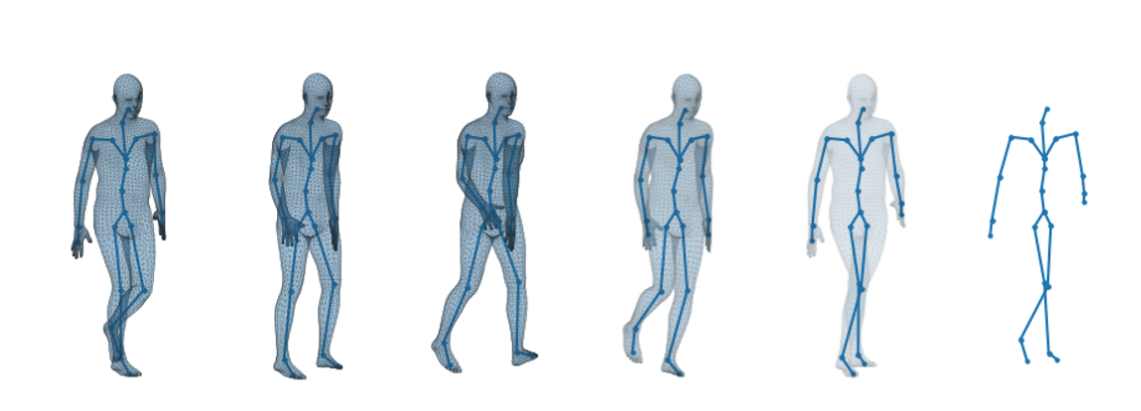
Human 3.6M (H3.6M) is a large-scale publicly available dataset including 3.6 million 3D motion-caption (abbreviated to mocap) data. H3.6M has constituted a widely used benchmark in human motion analysis and only recently new datasets started emerging.
The data consists of the recording of seven different actors performing 15 varied activities, such as walking, smoking, engaging in a discussion, and taking pictures. While performing these activities in front of multiple cameras, the humans wear a black jumpsuit with 41 markers taped on. The recordings are then processed to obtain a 3D representation of the movement in terms of markers position or joints-rotation for each frame.
Formally speaking, the input data ${X}$ is a sequence of length $T$ ,${(x_1, x_2, …, x_T)}$, where a frame $x_t \in{R^N}$ denotes the $N$-dimensional body pose.
$N$ depends on the number of joints in the skeleton, $K$, and the size $M$ of the per-joint representation, i.e. $N = K · M$.
A number of joint-representations have been proposed over the past few years and that of the representation scheme is a choice that has been and still is extensively discussed.
A quite common (and easy to come up with) representation is known as angle-axis or exponential maps: each joint is associated with an axis $w$ (for which you need 3 numbers), and an angle $\alpha$ (at least 3 more numbers in $R^3$). Usually, the input is standardized, discarding the information on the exact rotation vector of each joint, to focus on relative rotations between joints, since they contain information of the actions. Other representation schemes include rotation matrices, quaternions (we’ll get to this later), or 3D positions.
Problem formulation
Given a fixed length input sequence, as the one I’ve just introduced to you, the problem of human motion prediction can be phrased as the prediction of the future motion of the subject, both short-term and long-term. More formally, to goal of Human Motion Prediction is to find a mapping $P$ from an input sequence of length $T_1$ to an output sequence of length $T_2$.
Two different tasks
From the research on the field it has emerged that the short-term and the long-term prediction are two very different problems, and should hence be treated separately.
Historically, the best models on short-term prediction perform poorly on the long-term variant and vice versa. The reason for this is that while short-term prediction is mainly about completing a movement realistically (not breaking the rules of physics for instance), long-term prediction is more about being able to recognize and continue the intention of the human actor : if someone is about to make a phone call, you don’t expect them to start running, no matter how realistic the movement may seem!
Short-term tasks are hence often referred to as prediction tasks and can be assessed quantitatively by comparing the model prediction to a reference recording through a distance metric.
On the other hang long-term tasks are often referred to as generation tasks and are harder to assess quantitatively. For these cases, the prediction quality is usually evaluated by hand.
The papers
It’s finally time to dive into some of the most insightful deep-learning approaches in the history of the topic. In this section I am going to discuss 6 selected papers, focusing on their main contributions to the field.
#1 : On human motion prediction using recurrent neural networks
by Julieta Martinez, Michael J. Black, and Javier Romero.
I enjoyed reading this paper: the authors proposed many (though not too many) interesting ideas, that are clearly justified by a critical analysis of those that were state-of-the-art models in 2017. Too easily the scientific discourse can spiral down a dead-end, dragged by its own weight. Papers that can stir the discourse attention into a new direction, like this one, are necessary to its very progress.
The architecture
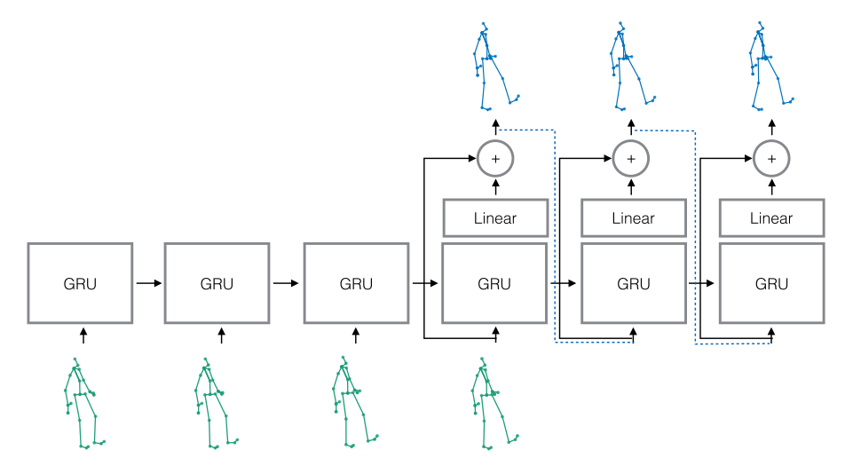
The architecture is a rather classic seq2seq model with GRU cells, with the addition of residual connections in the decoder and, interestingly, parameter sharing between encoder and decoder.
In seq2seq, two networks are trained;
(a) an encoder that receives the inputs and generates an internal representation, and
(b), a decoder network, that takes the internal state and produces a maximum likelihood estimate for prediction
Take-away points
The simplicity bias
The first and most elegant idea to take-away from this work is probably that of simplicity.
We have found a very simple baseline that outperforms sophisticated state-of-the-art methods based on deep RNNs for short-term motion prediction.
Simplicity has been a guideline to the development of this approach, and led the authors to at least three important choices:
- Avoiding solution whose effectiveness depend on the art of hyper-parameters tuning.
- Avoiding deeper and hence more computationally expensive models.
- Extending the specificity of the network.
And the experiments’ results show that this simplicity-biased mindset has repaid their trust, reporting new state-of-the-art results for the short-term motion prediction (up to 400 ms).
This simplicity-first approach also brought them to take into consideration an easy-to-implement but until then ignored baseline, which is still today hard to beat: the zero velocity baseline. Behind this fancy name is simply the concept of predicting zero movement, aka predicting stillness. To the surprise of the authors this baseline beated all state-of-the-art model back then:
We have found a very simple baseline that outperforms sophisticated state-of-the-art methods based on deep RNNs for short-term motion prediction.
Sampling-based loss
One of the problems that this model aims at solving is the typical incapacity of RNN models to recover from their own mistakes, which leads to a substantial discrepancy between training and testing performances, and hence to low robustness.
To address the issue they feed to the decoder its own samples, instead of the ground truth, at each training time-step.
Residual connections
This idea is the one that has brought the highest improvements on the results of their experiments, and it tackles the huge discontinuity between the conditioning sequence and prediction (aka between the first predicted frame and the last observed input).
The idea is simple and effective: instead of modelling all possible conditioning poses so that the first frame prediction is continuous, directly model the velocity of the model.
And to model velocity they propose a residual architecture, obtained by simply adding a residual connection between the input and the output of each RNN cell.
#2 : Learning Human Motion Models for Long-term Predictions
by Partha Ghosh, Jie Song, Emre Aksan, Otmar Hilliges
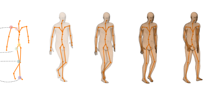
A fundamental issue that needs to be tackled when working with Human motion is that of constraining the prediction to a feasible subset of the output space. The skeletal constraints to human motion restrict the set of possible poses to a limited set. The problem arises when you need to force the predictions of your network into this subset.
In this paper Ghosh et al. give up on directly producing a correct prediction and instead focus on training a second network to correct the mistakes of the first one.
The architecture
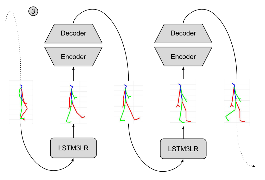
Figure 1 from the paper.
As I anticipated, the architecture is composed of two different networks: a recurrent network (LSTM3RL) and a de-noising auto-encoder (DAE). The former is responsible for the processing the input sequence and producing a prediction on the future sequence. Each frame of the LSTM3RL output is fed into the auto-encoder to be rectified.
LSTM3L is a classic recurrent network, with 3 layers of LSTM cells (hence the name 3RL), while DAE is an auto-encoder with increased dimensionality in the latent space.
The two components trained separately in order to de-correlate their errors and only once trained, they are fine-tuned in an end to end fashion.
Take-away points
Integrating domain knowledge
There’s still a question to solve: how can our de-noising auto-encoder incorporate domain knowledge?
The answer is, in my opinion, very ingenious and simple at the same time: dropout! The authors incorporated dropout in the DAE units, and hence trained it to reconstruct the input only by looking at a fraction of the total number of joints. This approach could not have worked if the joints were completely independent of one another: by randomly masking part of the input they forced the auto-encoder to learn the relationship between different joints.
With this training the DAE is then employed as a spatial filter: the corrupted pose predicted by the LSTM3RL network is first expanded into the latent space and then projected back into the input space by the decoder, which will recover an admissible spatial configuration.
No representation learning
An interesting point made by the authors of the paper is that there is no need to learn a condensed representation for the input in cases where it is already available in joint angle form.
The reasoning behind this claim is fairly straightforward:
[…] unlike image data, mocap data in its original representation is smooth and continuous while there exists no guarantees of these properties in the learnt latent space.
As a consequence, their model directly operates in joint-angle space, without pre-processing the input poses.
A metric for naturalness
Their third contribution worth mentioning is a metric to asses the naturalness of the pose. As I said before, there is no well-defined quantitative measure of the humans-faithfulness of a motion sequence (at least for now).
The authors circumnavigated the definition of a quantitative metric by training a separate classifier to predict the class to which the observed action belongs to. The idea is that the longer a sequence can be classified to belong to the same action category as the seed sequence the higher the quality of the prediction.
Again they managed to find a way to teach a network to do what before could by hand.
Similarities with previous works
The method described in this paper has two main contact points with Martinez et al. :
- The use of a sampling-based loss: at inference time Ghosh et al. feed back into the recurrent cell at time-step $t+1$ the output of the cell at time-step $t$ to give the model the chance to learn from its mistakes.
- The general-purpose network: following the steps of the before mentioned paper, the authors avoided training a task-specific model on each subtask by instead training a single, general-purpose model.
#3 : Modeling Human Motion with Quaternion-based Neural Networks
by Dario Pavllo, Christoph Feichtenhofer, Michael Auli, David Grangier
This paper extensively explores the weaknesses of the available representations for three-dimensional poses and extends the domain making use of a new abstraction: the quaternion.
I will not discuss the architecture for this paper because I believe that the main source of innovation here is in the in-depth analysis of the representation problem.
Quaternions?
Let me first clear out any source of confusion. Although the name evokes some sort of esoteric concept, quaternions are just 4-tuples. As Wikipedia puts it :
Quaternions are a number system that extends the complex numbers. […]
Quaternions are generally represented in the form $a + bi + cj + dk$, where $a, b, c$, and $d$ are real numbers, and $i, j$, and $k$ are the fundamental quaternion units.

The question running through your head at this point might be something along the line:
What do quaternions have to do with human motion?
To answer this question, let me first present to you the major shortcomings of the other available representations. Before quaternions were first introduced as a viable alternative two widely used parametrization schemes for rotations in the 3D Euclidean space were Euler angles and Exponential maps.
Euler angles represent orientations as successive rotations around the axes of a coordinate system. As you might guess, there are multiple ways to compose rotations in order to obtain the same final result. This is why applications that use Euler angles must agree on the particular order convention. A typical Euler rotation vector is a triplet that indicates the rotation around each axis in radians. There are two drawbacks in adopting a Euler angles representation:
- Each rotation is not uniquely identified, since $x$ and $x + 2\pi$ represent the same angle;
- The representation space is discontinuous, since it jumps back to $0$ every time the rotation angle reaches $2\pi$.
The exponential map parametrization scheme, also known as axis angle representation was proposed as a more practical alternative to Euler angles. Intuitively, an axis-angle rotation is described by an axis $\hat{e}$ (a 3D unit vector) and a rotation angle $\theta$ around this axis. I am sorry to disappoint you, but exponential maps have the same weaknesses of Euler angles, namely:
- Singularities in the representation;
- Discontinuity in the parameter space.
- There is also a third issue with the exponential map representation:
Multiple rotations cannot be composed into one single rotation. This is maybe the most annoying disadvantage when it comes to apply such a parametrization in the field of human motion prediction, since composition is a fundamental operator for forward kinematics.
Now we have enough material to justify quaternions in the context of human motion modeling. Analogously to exponential maps, quaternions describe a 3D rotation with an angle $\theta$ and an axis $\hat{e}$. A rotation of $\theta$ radians around an axis $\hat{e}$ is encoded as a = $cos(\theta/2)$ and $bcd = \hat{e}\sin(\theta/2)$. This representation has multiple features that help it overcome the above mentioned limitations of the alternatives. I’ll summarize its advantages in the following list:
- No singularities: each rotation is uniquely identified with a quaternion representation.
- No discontinuities in the parameter space: this is particularly useful when regressing on rotations.
- Fully composable : in the quaternions domain rotations can be composed and used to compute transformations.
- Interpolation: quaternions are also surprisingly handy to perform interpolation between rotations.
- Numerical stability: last but not least, quaternion based parametrization schemes are numerically stable, and are more computationally efficient than other representations.
So far so good. Unfortunately, quaternions have disadvantages too. The main issue when quaternions arises from the so-called antipodal representations: two opposite quaternions $q$ and $-q$ describe the same 3D rotation. Nevertheless, this dual parametrization represents improvement over the infinite set of equivalent representations in the Euler angles and exponential maps space.
This was it for quaternions, now let’s proceed with the next paper.
#4: Adversarial Geometry-Aware Human Motion Prediction
by Liang-Yan Gui, Yu-Xiong Wang, Xiaodan Liang, and Jos´e M. F. Moura
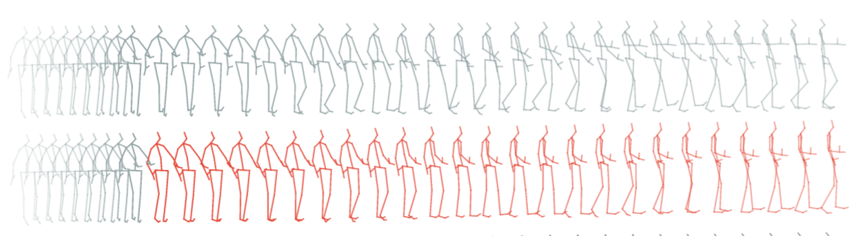
Finally we discuss one of the most influential and successful papers on human motion prediction. The Adversarial Geometry-Aware Encoder-Decoder model (abbreviated AGED) reached SOTA results at the time of publication. The approach proposed in this paper builds mainly upon the work of Martinez et al., enriching the solution with the surprisingly powerful adversarial framework.
Although this work markedly outperformed the previous approaches its contribution can be seen as limited to the loss definition problem. The authors tackled both the frame-level and sequence-level loss. This remarkable result sheds a light on the already-known-to-be fundamental role of the loss in machine learning problems.
The architecture
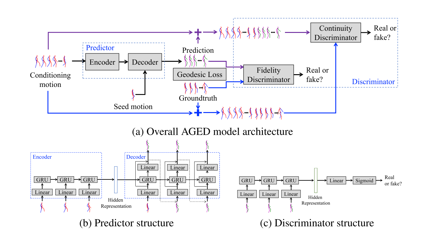
I have to admit that at first sight the architecture design might seem complicated. However, as you’ll soon discover by yourself, the idea is easy to grasp and also makes a lot of sense.
In every adversarial framework there must be generator and a discriminator.
As a generator the authors use an auto-encoder similar to the one discussed in Martinez et al. The network is trained to minimize the Geodesic distance between prediction and ground-truth at the frame level. In the next section I’ll discuss the meaning of this specific distance, for now just think of it as an alternative to the more familiar Euclidean distance. The encoder will learn to extract a lower dimensional representation of the input sequence, while the decoder will learn to produce a prediction given a seed motion frame and the encoded version of the input. Again following Martinez et al.’s footsteps the authors make use of residual connections in the decoder architecture.
As you can see from the above schema, the model comprises two different discriminators: a fidelity discriminator and a continuity discriminator (I’ll later explain the motivation behind these two names). Both discriminators are recurrent networks, with a dense head on top to produce a binary output.
Take-away points
A geodesic loss
The idea is to find a distance measure that is specific to rotations. The Euclidean measure treats the rotation coordinates as ordinary points in a 3D space. Rotations implicitly encode geometric information which should not be discarded when computing the loss.
The Geodesic distance measures the shortest path between two rotations, and is hence able to capture the inherent geometric structure of rotations. Such a geometrically more meaningful loss leads to more precise distance measurement, with the advantage of being computationally inexpensive.
Interestingly enough, the geodesic distance “it’s fully equivalent to the quaternion based metric”. However, computationally speaking, the authors claim that “experimental results” indicate that “the quaternion based metric led to worse results, possibly due to the need for renormalization of quaternions during optimization”.
A sequence-level loss
The issue that’s being tackled here is the same that Ghosh et al. addressed with their metric for naturalness. As I anticipated in the introduction, it’s hard to evaluate quantitatively the quality of the predictions. However, it’s fairly easy to argue that a measure of “plausibility” is ultimately a necessary ingredient in a network whose goal is to generate “good-looking” sequences. Using the authors’ argument:
This is partially because using a frame-wise regression loss solely cannot check the fidelity of the entire predicted sequence from a global perspective.
Their solution is similar in spirit to that of Ghosh et al., in the sense that both avoided the hard problem of explicitly defining such a measure by instead training an additional network to play the part of the critic. The differences between the two approaches stems from the way the two model’s components were connected. While Ghosh et al. ended up pipelining the two networks in a collaborative fashion, here Gui et al. adopted an adversarial approach, forcing the generator and the two discriminators to compete against each other.
Let’s first talk about the fidelity discriminator.
This component is fed ground truth and generated sequences in an alternating fashion, and it’s trained to correctly identify original and fake inputs. The idea is that such a discriminator should be able to examine whether the generated motion sequence is human-like and plausible overall.
Now to the continuity discriminator.
This second network is given as input the concatenation of the conditioning sequence (the frames based on which the generator makes a prediction) and the true and fake future frames, again in an alternating fashion. The continuity discriminator hence gets to observe the motion from the beginning at time step $0$ until the very end at time step $T_1 + T_2$, where $T_1$ is the length of the input and $T_2$ is the desired length of the output, while the fidelity discriminator only receives the frames from time step $T_1$ to $T_2$.
Intuitively, being trained on this extended version of the sequence, the continuity discriminator should learn to check whether the predicted motion sequence is coherent with the input sequence without a noticeable discontinuity between them.
The idea should be evident by now: the quality of the predictions from an overall perspective can be assessed by indirectly looking at the two discriminators. The better the generator is at fooling the two adversaries, the more human-like and coherent the predicted frames should seem to a human.
We can finally put together everything we’ve learned so far and look at the objective of the model, which is obtained by integrating the geodesic loss and the two adversarial losses:
#5 : Learning Trajectory Dependencies for Human Motion Prediction
by Wei Mao, Miaomiao Liu, Mathieu Salzmann, Hongdong Li
To understand the solution proposed here we first need to take a step back and do a brief recap of the problem.
As stated in the introduction section, human motion modeling is about predicting $T_2$ future motion frames, given $T_1$ past frames as input. At each time-step we get to observe either the absolute position or the relative rotation of each modeled joint. Taking a step further, looking at each joint separately we would observe its trajectory.
Centuries of signal processing math tell us that any sequence in the time domain can be analysed as well in the frequency domain by accessing its spectrum. For those not familiar with these concepts, you can think of the frequency of a signal as an indicator of the rapidity of changes in it. To the beauty of this dualism contributes the fact that the two representations are exactly equivalent, i.e. there is no loss of information in going from one to another.
Hypothetically speaking then it should be possible to represent the movements of each joint in the frequency domain using its spectrum. In this paper Mao et al. experiment with precisely this idea: flipping over the perspective by looking at the joints’ frequencies instead of the joints’ positions.
The architecture
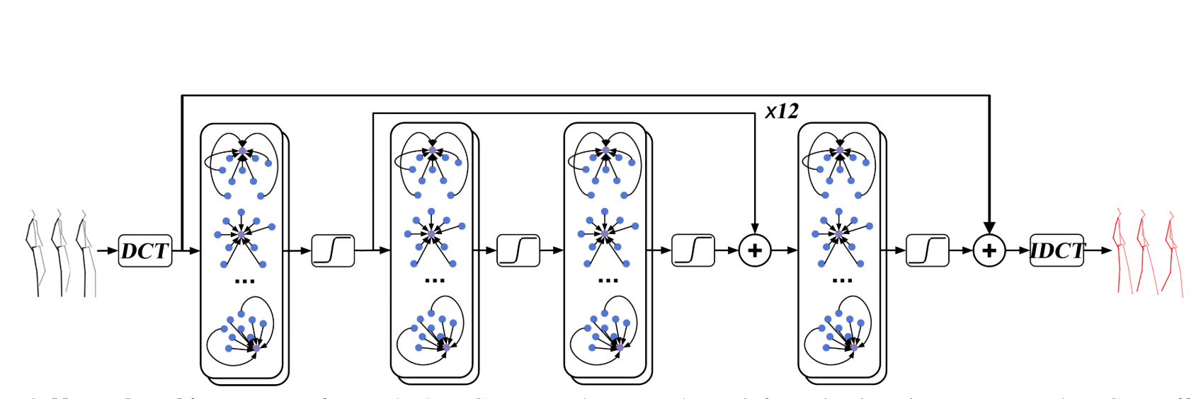
As depicted in the architecture’s scheme above, the signal is first passed through the Discrete Cosine Transform (DCT) block: this is where the perspective is flipped, i.e. where we compute the spectrum for each single joint. The spectrum consists in a series of coefficients, identifying the principal frequencies in the input signal (more on this in the next section). To get our predictions back in the time domain we then pass the predicted coefficients trough an Inverse Discrete Cosine Transform block (IDCT as visible in the scheme) at the end of the pipeline.
To generate predictions in the frequency domain the authors resorted to the use of residual connections and graph convolutional networks. More precisely, these middle layers consist of 12 residual blocks, each of which comprises 2 graph convolutional layers, and two additional graph convolutional layers.
The use of residual connections should by now sound familiar: the authors admittedly drew inspiration from the work of Martinez et al., applying the zero-velocity baseline idea to the frequency space.
On the other hand, graph convolutional networks are pure novelty in the context of human motion prediction: the idea is to capture the spatial structure of the motion data by learning a graph representation for it.
Take-away points
A feed-forward approach
Differently from all previous approaches, Mao et al. refrain from resorting to a sequential model by instead working in the trajectory space with a simple yet effective feed-forward model. As I mentioned previously, to encode the temporal nature of human motion the authors adopt a trajectory representation based on the Discrete Cosine Transform.
Let us denote by \(x^k = x^{k}_1, x^{k}_2, x^{k}_3, ... , x^{k}_N\) the trajectory for the $k$ th joint across $N$ frames. […]
To make use of the DCT representation, instead of treating motion prediction as the problem of learning a mapping from $X_{1:N}$ to $X_{N+1:N+T}$, we reformulate it as one of learning a mapping between observed and future DCT coefficients.
The data in the frequency domain undergoes an additional pre-processing step, which turns out to be a smart (and easy to implement) solution to increase the quality of the predictions. The idea is simply to filter the spectrum of the signal by discarding the frequencies above a certain threshold, a well known concept in signal-processing called low-pass filtering. The main motivation behind this is that, by discarding the high frequencies, the DCT can nicely capture the smoothness of human motion.
Graph convolutions
Graph convolutions have first been proposed in 2016 and 2017. The idea is still in its early stages but it’s nonetheless powerful. For those of you that are reading the term Graph Convolutional Networks (GCN) for the first time, you can think of it as a convolution operator that instead of working with raw vectors can be applied to graphs.
In this work, Mao et al. employ GCNs to treat the human pose as a generic graph (rather than a human skeletal kinematic tree) formed by links between every pair of body joints. Instead of using a pre-defined graph structure, the authors design a new graph convolutional network to learn graph connectivity automatically. This allows the network to capture long range dependencies beyond that of human kinematic tree.
Moreover, each of the GCN layers in the model has an independent structure. Using a different learnable adjacency matrix for every graph convolutional layer allows the network to adapt the connectivity for different operations.
The novelty
This is probably the most groundbreaking and innovational paper of the series. In my opinion, not only the authors managed to contribute to the scientific discourse with a smart and successful solution, but also and above all they introduced a drastically different way of framing the problem, effectively opening new directions to the future developments on the topic of human motion prediction.
The scientific community usually tends to spiral around the most promising approach, rarely focusing on alternatives. I hence consider praiseworthy (and essential) the research that is able to jump off the leading train to embrace a yet unexplored and much less favorable path.
#6 : Structured Prediction Helps 3D Human Motion Modelling
by Emre Aksan, Manuel Kaufmann, Otmar Hilliges
We have finally reached the last of the six papers that I’ve selected for this discussion.
Do not expect to see a new architecture though, because the contribution of this work mainly revolves around a a novel structured prediction layer (SPL) that can be incorporated by any of the approaches we’ve discussed so far. The experiments carried on by the authors show a marked improvement in the performance of existing models when including the SP-layer.
The idea behind the SP-layer is to model the structure of the human skeleton and hence the spatial dependencies between joints. The approach is motivated by the observation that human motion is strongly regulated by the spatial structure of the skeleton.
As it happens with any statistical tool, incorporating domain knowledge (usually in the form of priors) can drastically improve the model’s performance - if the prior is correct. The hypothesis which is being addressed by the authors can hence be summarized as follows:
Successfully exploiting spatial priors in human motion modelling can in turn allow recurrent models to capture temporal coherency more effectively.
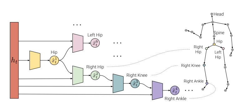
A structure prediction layer
The SP-layer models the the spatial dependencies between joints via a hierarchy of small-sized neural networks that are connected analogously to the kinematic chains of the human skeleton. Each node in the graph receives information about the parent node’s prediction and thus information is propagated along the kinematic chain.
The figure above shows the internal structure of the SP-layer.
The input $h_t$ is a generic context representation, i.e. a vector which is assumed to summarize the motion sequence until time $t$. While the previously discussed architectures leverage several dense layers to predict the whole $N$-dimensional pose vector $x_t$ given $h_t$, the SP-layer predicts each joint individually with separate smaller networks.
Because the per-joint decomposition leads to many small separate networks, we can think of an SP-layer as a dense layer where some connections have been set to zero explicitly by leveraging domain knowledge.
Formally speaking, the above scheme defines a Bayesian network over the joints positions from which we can extract a factorized version of the “joint distribution” via the chain rule, i.e. :
Note that each sub-layer is receiving as input both the parents’ predictions and the context vector. In this formulation each joint receives information about its own configuration and that of the immediate parent both explicitly, through the conditioning on the parent joint’s prediction, and implicitly via the context.
As an example, unrolling the above equation with respect to the scheme shown above we would get something along the line:
\[p_\theta(x_t) = p_\theta(\, x_t^{(hip)} \, | \,h_t)\,p_\theta(\, x_t^{(spine)} \, |\, x_t^{(hip)}, \,h_t\,)\, ...\]
The benefit of this structured prediction approach is twofold.
- Saving model capacity: the proposed factorization allows for integration of a structural prior in the form of a hierarchical architecture where each joint is modelled by a different network. This allows the model to learn dedicated representations per joint and hence saves model capacity.
- Increasing precision: analogous to message passing, each parent propagates its prediction to the child joints, allowing for more precise local predictions because the joint has access to the information it depends on (i.e., the parent’s prediction).
Additionally, the authors propose a similar decomposition in the objective function, giving birth to a new per joint loss. Instead of calculating the error on every frame and then summing over the time steps in the sequence, Aksan et al. directly calculate the error on each joint separately, summing the results across both temporal and spatial domain.
As we’ve got to see through the previous works, the loss is an extensively discussed topic in the context of human motion prediction, since its definition can sensibly influence the outcome of an experiment.
The end
This is it for today: our journey through human motion prediction stops here.
Nonetheless, the topic continues to evolve as the ability of interacting with complex human environment is perceived as essential by an increasing number of applications.
Here’s a beautiful quote that I’d like to end this discussion with:
Any sufficiently advanced technology is indistinguishable from magic.
― Arthur C. Clarke, Profiles of the Future: An Inquiry Into the Limits of the Possible
References
If you want to continue the journey on your own here are some links that you might find useful:
[1] Martinez et al. (2017) On Human Motion Prediction Using Recurrent Neural Networks
[2] Ghosh et al. (2017) Learning Human Motion Models for Long-term Predictions
[3] Pavllo et al. (2018) Modeling human motion with quaternion-based neural networks
[4] Wang et al. (2018) Adversarial geometry-aware human motion prediction
[5] Mao et al. (2019) Learning Trajectory Dependencies for Human Motion Prediction
[6] Aksan et al. (2019) Structured Prediction Helps 3D Human Motion Modelling